The Distribution of Linear Regression Coefficients
| ... from pacal import *
|
||
|
.
|
||
Using compiled interpolation routine
Compiled sparse grid routine not available
| ... from pylab import figure, show, plot, subplot, title
from scipy.optimize import fmin
from numpy.random import seed
from numpy import concatenate, polyfit, array
seed(1)
import time
t0 = time.time()
params.interpolation_nd.maxq = 7
params.interpolation.maxn = 50
params.interpolation_pole.maxn = 50
params.interpolation_finite.maxn = 50
params.interpolation_infinite.maxn = 50
params.interpolation.debug_info = False
params.interpolation_nd.debug_info = False
params.models.debug_info = True
|
||
|
.
|
||
Sample
| ... n=10
#Xobs = UniformDistr().rand(n)
a, b = 0.3, 0.7
#Ei = NormalDistr(0.0,0.25) | Between(-1,1)
#Yobs = a * Xobs + b + Ei.rand(n)
Xobs=array([ -0.165955990595, 0.440648986884, -0.999771250365, -0.395334854736, -0.706488218366, -0.815322810462, -0.627479577245, -0.308878545914, -0.206465051539, 0.0776334680067 ])
Yobs=array([ 0.599227844272, 0.952772646868, 0.193629370472, 0.872776787585, 0.00800832135878, 0.565696815404, 0.459561157571, 0.644246153468, 0.368440390549, 0.511201707273 ])
print '{0:{align}15}\t{0:{align}15}'.format("Xobs","Xobs", align = '>')
|
||
|
.
|
||
Xobs Xobs
| ... for i in range(len(Xobs)):
print '{0:{align}20}\t{0:{align}14}'.format(Xobs[i], Yobs[i], align = '>')
|
||
|
.
|
||
-0.165955990595        0.599227844272
 0.440648986884        0.952772646868
-0.999771250365        0.193629370472
-0.395334854736        0.872776787585
-0.706488218366        0.00800832135878
-0.815322810462        0.565696815404
-0.627479577245        0.459561157571
-0.308878545914        0.644246153468
-0.206465051539        0.368440390549
0.0776334680067        0.511201707273
| ... print "x=c(", ", ".join(str(x) for x in Xobs), ")"
|
||
|
.
|
||
x=c( -0.165955990595, 0.440648986884, -0.999771250365, -0.395334854736, -0.706488218366, -0.815322810462, -0.627479577245, -0.308878545914, -0.206465051539, 0.0776334680067 )
| ... print "y=c(", ", ".join(str(x) for x in Yobs), ")"
|
||
|
.
|
||
y=c( 0.599227844272, 0.952772646868, 0.193629370472, 0.872776787585, 0.00800832135878, 0.565696815404, 0.459561157571, 0.644246153468, 0.368440390549, 0.511201707273 )
Model
| ... X = []
E = []
Y = []
#A = UniformDistr(0,1, sym = "A")
A = UniformDistr(-0.5, 1.5, sym = "A")
B = UniformDistr(-0.0, 1.5, sym = "B")
#A = NormalDistr(0.0,0.2) | Between(-1,1)
#B = NormalDistr(0.0,0.2) | Between(-1,1)
for i in range(n):
X.append(UniformDistr(-1, 1, sym = "X{0}".format(i)))
E.append(NormalDistr(0.0,0.2) | Between(-1.0,1.0))
E[i].setSym("E{0}".format(i))
Y.append(A * X[i] + B + E[i])
Y[i].setSym("Y{0}".format(i))
M = Model(X + E + [A, B], Y)
M.toGraphwiz(f=open('bn.dot', mode="w+"))
print M
|
||
|
.
|
||
Model:
free_vars:
   A ~ U(-0.5,1.5)
   B ~ U(-0.0,1.5)
   E0 ~ N(0.0,0.2) | X>-1.0 | X<1.0
   E1 ~ N(0.0,0.2) | X>-1.0 | X<1.0
   E2 ~ N(0.0,0.2) | X>-1.0 | X<1.0
   E3 ~ N(0.0,0.2) | X>-1.0 | X<1.0
   E4 ~ N(0.0,0.2) | X>-1.0 | X<1.0
   E5 ~ N(0.0,0.2) | X>-1.0 | X<1.0
   E6 ~ N(0.0,0.2) | X>-1.0 | X<1.0
   E7 ~ N(0.0,0.2) | X>-1.0 | X<1.0
   E8 ~ N(0.0,0.2) | X>-1.0 | X<1.0
   E9 ~ N(0.0,0.2) | X>-1.0 | X<1.0
   X0 ~ U(-1,1)
   X1 ~ U(-1,1)
   X2 ~ U(-1,1)
   X3 ~ U(-1,1)
   X4 ~ U(-1,1)
   X5 ~ U(-1,1)
   X6 ~ U(-1,1)
   X7 ~ U(-1,1)
   X8 ~ U(-1,1)
   X9 ~ U(-1,1)
dep vars:  X61312592(2), X61359024(2), X61361616(2), X61735696(2), X61761008(2), X61761424(2), X61788080(2), X61820848(2), X61849264(2), X61872944(2), X61358160(11), Y0(11), Y1(11), X61361424(11), X61374192(11), Y2(11), Y3(11), X61737808(11), Y4(11), X61762960(11), X61786384(11), Y5(11), Y6(11), X61819760(11), Y7(11), X61848176(11), Y8(11), X61872752(11), X61899920(11), Y9(11)
Equations:
X61358160 = B + X61312592(11)
X61786384 = B + X61761424(11)
Y0 = E0 + X61358160(11)
Y5 = E5 + X61786384(11)
Y3 = E3 + X61737808(11)
Y6 = E6 + X61819760(11)
X61848176 = B + X61820848(11)
Y8 = E8 + X61872752(11)
X61735696 = A*X3(2)
X61872944 = A*X9(2)
X61737808 = B + X61735696(11)
X61819760 = B + X61788080(11)
Y1 = E1 + X61361424(11)
X61359024 = A*X1(2)
X61361424 = B + X61359024(11)
Y7 = E7 + X61848176(11)
Y4 = E4 + X61762960(11)
X61899920 = B + X61872944(11)
Y9 = E9 + X61899920(11)
X61762960 = B + X61761008(11)
X61361616 = A*X2(2)
X61761008 = A*X4(2)
X61820848 = A*X7(2)
X61312592 = A*X0(2)
X61849264 = A*X8(2)
X61374192 = B + X61361616(11)
Y2 = E2 + X61374192(11)
X61761424 = A*X5(2)
X61872752 = B + X61849264(11)
X61788080 = A*X6(2)
Factors:
F_0 (X0)<class 'pacal.depvars.nddistr.Factor1DDistr'>
F_1 (X1)<class 'pacal.depvars.nddistr.Factor1DDistr'>
F_2 (X2)<class 'pacal.depvars.nddistr.Factor1DDistr'>
F_3 (X3)<class 'pacal.depvars.nddistr.Factor1DDistr'>
F_4 (X4)<class 'pacal.depvars.nddistr.Factor1DDistr'>
F_5 (X5)<class 'pacal.depvars.nddistr.Factor1DDistr'>
F_6 (X6)<class 'pacal.depvars.nddistr.Factor1DDistr'>
F_7 (X7)<class 'pacal.depvars.nddistr.Factor1DDistr'>
F_8 (X8)<class 'pacal.depvars.nddistr.Factor1DDistr'>
F_9 (X9)<class 'pacal.depvars.nddistr.Factor1DDistr'>
F_10 (E0)<class 'pacal.depvars.nddistr.Factor1DDistr'>
F_11 (E1)<class 'pacal.depvars.nddistr.Factor1DDistr'>
F_12 (E2)<class 'pacal.depvars.nddistr.Factor1DDistr'>
F_13 (E3)<class 'pacal.depvars.nddistr.Factor1DDistr'>
F_14 (E4)<class 'pacal.depvars.nddistr.Factor1DDistr'>
F_15 (E5)<class 'pacal.depvars.nddistr.Factor1DDistr'>
F_16 (E6)<class 'pacal.depvars.nddistr.Factor1DDistr'>
F_17 (E7)<class 'pacal.depvars.nddistr.Factor1DDistr'>
F_18 (E8)<class 'pacal.depvars.nddistr.Factor1DDistr'>
F_19 (E9)<class 'pacal.depvars.nddistr.Factor1DDistr'>
F_20 (A)<class 'pacal.depvars.nddistr.Factor1DDistr'>
F_21 (B)<class 'pacal.depvars.nddistr.Factor1DDistr'>
Inference
| ... MAB = M.inference([A,B], X + Y, concatenate((Xobs, Yobs)))
|
||
|
.
|
||
condition on variable:  X0 = -0.165955990595
condition on variable:  X1 = 0.440648986884
condition on variable:  X2 = -0.999771250365
condition on variable:  X3 = -0.395334854736
condition on variable:  X4 = -0.706488218366
condition on variable:  X5 = -0.815322810462
condition on variable:  X6 = -0.627479577245
condition on variable:  X7 = -0.308878545914
condition on variable:  X8 = -0.206465051539
condition on variable:  X9 = 0.0776334680067
exchange free variable:  A with dependent variable X61312592
exchange free variable:  X61312592 with dependent variable X61359024
exchange free variable:  X61359024 with dependent variable X61361616
exchange free variable:  X61361616 with dependent variable X61735696
exchange free variable:  X61735696 with dependent variable X61761008
exchange free variable:  X61761008 with dependent variable X61761424
exchange free variable:  X61761424 with dependent variable X61788080
exchange free variable:  X61788080 with dependent variable X61820848
exchange free variable:  X61820848 with dependent variable X61849264
exchange free variable:  X61849264 with dependent variable X61872944
exchange free variable:  B with dependent variable X61358160
exchange free variable:  E0 with dependent variable Y0
condition on variable:  Y0 = 0.599227844272
exchange free variable:  X61358160 with dependent variable X61361424
exchange free variable:  E1 with dependent variable Y1
condition on variable:  Y1 = 0.952772646868
exchange free variable:  X61361424 with dependent variable X61374192
exchange free variable:  E2 with dependent variable Y2
condition on variable:  Y2 = 0.193629370472
exchange free variable:  X61374192 with dependent variable X61737808
exchange free variable:  E3 with dependent variable Y3
condition on variable:  Y3 = 0.872776787585
exchange free variable:  X61737808 with dependent variable X61762960
exchange free variable:  E4 with dependent variable Y4
condition on variable:  Y4 = 0.00800832135878
exchange free variable:  X61762960 with dependent variable X61786384
exchange free variable:  E5 with dependent variable Y5
condition on variable:  Y5 = 0.565696815404
exchange free variable:  X61786384 with dependent variable X61819760
exchange free variable:  E6 with dependent variable Y6
condition on variable:  Y6 = 0.459561157571
exchange free variable:  X61819760 with dependent variable X61848176
exchange free variable:  E7 with dependent variable Y7
condition on variable:  Y7 = 0.644246153468
exchange free variable:  X61848176 with dependent variable X61872752
exchange free variable:  E8 with dependent variable Y8
condition on variable:  Y8 = 0.368440390549
exchange free variable:  X61872752 with dependent variable X61899920
exchange free variable:  E9 with dependent variable Y9
condition on variable:  Y9 = 0.511201707273
exchange free variable:  X61872944 with dependent variable A
exchange free variable:  X61899920 with dependent variable B
| ... params.interpolation.maxn = 100
params.interpolation_pole.maxn = 100
MA = MAB.inference([A],[],[])
MB = MAB.inference([B],[],[])
print MAB
|
||
|
.
|
||
Model:
free_vars:
   A ~ U(-0.5,1.5)
   B ~ U(-0.0,1.5)
dep vars:
Equations:
Factors:
F_0 (A)<class 'pacal.depvars.nddistr.NDDistrWithVarSubst'>
F_1 (B,A)<class 'pacal.depvars.nddistr.NDDistrWithVarSubst'>
F_2 (B,A)<class 'pacal.depvars.nddistr.NDDistrWithVarSubst'>
F_3 (B,A)<class 'pacal.depvars.nddistr.NDDistrWithVarSubst'>
F_4 (B,A)<class 'pacal.depvars.nddistr.NDDistrWithVarSubst'>
F_5 (B,A)<class 'pacal.depvars.nddistr.NDDistrWithVarSubst'>
F_6 (B,A)<class 'pacal.depvars.nddistr.NDDistrWithVarSubst'>
F_7 (B,A)<class 'pacal.depvars.nddistr.NDDistrWithVarSubst'>
F_8 (B,A)<class 'pacal.depvars.nddistr.NDDistrWithVarSubst'>
F_9 (B,A)<class 'pacal.depvars.nddistr.NDDistrWithVarSubst'>
F_10 (B,A)<class 'pacal.depvars.nddistr.NDDistrWithVarSubst'>
F_11 (B,A)<class 'pacal.depvars.nddistr.NDDistrWithVarSubst'>
F_12 ()<class 'pacal.depvars.nddistr.NDConstFactor'>
| ... print MA
|
||
|
.
|
||
Model:
free_vars:
   A ~ U(-0.5,1.5)
dep vars:
Equations:
Factors:
F_0 (A)<class 'pacal.depvars.nddistr.NDDistrWithVarSubst'>
F_1 (A)<class 'pacal.depvars.nddistr.NDInterpolatedDistr'>
F_2 ()<class 'pacal.depvars.nddistr.NDConstFactor'>
| ... print MB
|
||
|
.
|
||
Model:
free_vars:
   B ~ U(-0.0,1.5)
dep vars:
Equations:
Factors:
F_0 (B)<class 'pacal.depvars.nddistr.NDInterpolatedDistr'>
F_1 ()<class 'pacal.depvars.nddistr.NDConstFactor'>
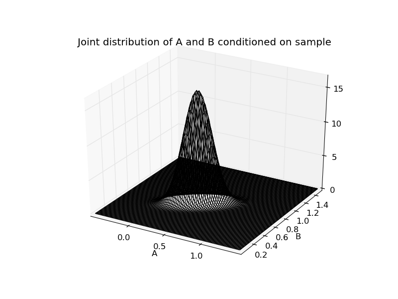
| ... figure(1)
MAB.plot(have_3d=True)
title("Joint distribution of A and B conditioned on sample")
show()
|
||
|
.
|
||
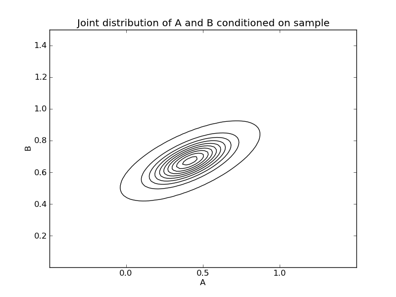
| ... figure(2)
MAB.plot(have_3d=False, cont_levels=10)
title("Joint distribution of A and B conditioned on sample")
show()
|
||
|
.
|
||
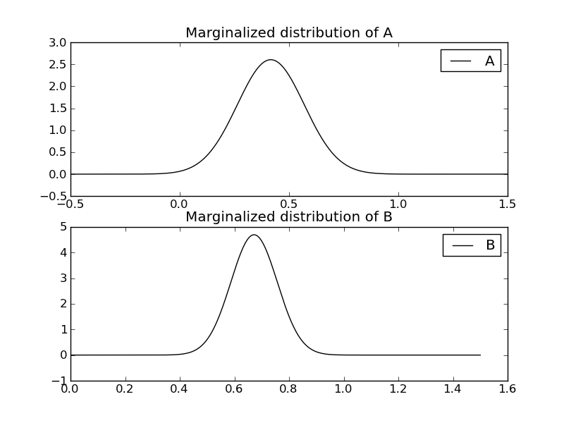
| ... figure(3)
subplot(211)
MA.plot()
|
||
|
.
|
||
============= summary =============
  FUN(-0.5,1.5)
                mean  =  0.41645355509034099
                 var  =  0.023464241392269252
            skewness  =  -3.7665393628279955e-08
            kurtosis  =  2.9999985597715617
             entropy  =  -0.45720036463886982
              median  =  0.4164535332421927
                mode  =  0.41645353919269024
            medianad  =  0.10331862001613233
      iqrange(0.025)  =  0.6004561331294082
            ci(0.05)  =  (0.11622542905463824, 0.7166815621840464)
               range  =  (-0.5, 1.5)
             tailexp  =  (None, None)
             int_err  =  -3.4207779275874373e-08
| ... title("Marginalized distribution of A")
subplot(212)
MB.plot()
|
||
|
.
|
||
============= summary =============
  FUN(-0,1.5)
                mean  =  0.67195270604723933
                 var  =  0.0072251407656638185
            skewness  =  -7.8840675802035367e-07
            kurtosis  =  2.9999995867207456
             entropy  =  -1.0461558406701483
              median  =  0.6719526773756899
                mode  =  0.67195268094315619
            medianad  =  0.057332184251915205
      iqrange(0.025)  =  0.33319706834906826
            ci(0.05)  =  (0.5053541212593485, 0.8385511896084168)
               range  =  (-0, 1.5)
             tailexp  =  (None, None)
             int_err  =  -3.6473167597250722e-08
| ... title("Marginalized distribution of B")
show()
|
||
|
.
|
||
Estimation of coefficients
| ... print "original coefficients a=", a, "b=", b
|
||
|
.
|
||
original coefficients a= 0.3 b= 0.7
| ... print "mean est. A=", MA.as1DDistr().mean(), "est. B=", MB.as1DDistr().mean()
|
||
|
.
|
||
mean est. A= 0.41645355509 est. B= 0.671952706047
| ... print "median est. A=", MA.as1DDistr().median(), "est. B=", MB.as1DDistr().median()
|
||
|
.
|
||
median est. A= 0.416453533242 est. B= 0.671952677376
| ... print "mode est. A=", MA.as1DDistr().mode(), "est. B=", MB.as1DDistr().mode()
|
||
|
.
|
||
mode est. A= 0.416453539193 est. B= 0.671952680943
| ... print MA.as1DDistr().cdf(0.0)
|
||
|
.
|
||
0.00327682546711
| ... print MB.as1DDistr().cdf(0.0)
|
||
|
.
|
||
0.0
| ... MAB.nddistr(1, 3)
abopt = MAB.nddistr.mode()
|
||
|
.
|
||
Warning: Desired error not necessarily achieved due to precision loss
         Current function value: -16.428083
         Iterations: 31
         Function evaluations: 2291
         Gradient evaluations: 524
| ... (ar,br)=polyfit(Xobs,Yobs,1)
|
||
|
.
|
||
Least squares estimates are maximum log-likelihood estimates (are equal to maximum a posteriori in this case, because of uniform a priori distribution of coefficients)
| ... print " MAP a=", abopt[0], "b=", abopt[1]
|
||
|
.
|
||
MAP a= 0.416453467936 b= 0.671952615709
| ... print "polyfit (LSE) est. a=", ar, "b=", br
|
||
|
.
|
||
polyfit (LSE) est. a= 0.416453539158 b= 0.671952681142
| ... print "computation time=", time.time() - t0
|
||
|
.
|
||
computation time= 154.951999903
| ... |
||
|
.
|
||